

{{quote1}}
Why build this?
Imagine you are a fraud analyst at a fintech. You have just spotted a new pattern:
Flag any payment where a new beneficiary receives more than €5,000 in the last 24 hours.
In many systems, turning that insight into a production rule means:
- talking to engineers
- designing a new index
- waiting for it to build and be rolled out safely
By the time the rule is live, the pattern may have changed.
At Marble, customers define their own data model and their own aggregates. We wanted analysts to:
- add or change aggregates on their own
- push new rule versions to production
- have the system automatically build the right indexes for good performance
We solved this with an opinionated, data-agnostic algorithm that turns arbitrary aggregate queries into a small set of PostgreSQL indexes, with automatic creation and cleanup.
Context: building aggregates on a custom data model
Marble is a decision engine for fraud and AML. Customers:
- define a custom schema (tables, columns, relations)
- ingest their own data
- write rules that reference aggregates over that data
We store customer data in PostgreSQL, typically with:
- one dedicated schema per organization (for example
org_data) - multiple tables, such as
transactions,accounts, andusers - informal foreign keys between tables (known to Marble, not enforced by Postgres)
For simplicity, assume we have:
- schema:
org_data - tables:
transactions,accounts,users - high-volume table:
transactions(millions of rows per month) - lower-volume tables:
accounts,users(thousands of rows)
Rules can reference aggregates such as:
- onboarding:
- number of existing customers sharing the same name or address
- transaction monitoring:
- sum of payments made to a given beneficiary over the last 30 days
- number of payments with a suspicious label similar to the current one
- count of cross-border payments this month above a given threshold
Filters can also depend on runtime values (payload fields, allowlists, and similar). For a query such as:
SELECT SUM(amount)
FROM org_data.transactions
WHERE account_id = $1
AND transaction_at > $2
AND transaction_at < $3
AND payment_method = $4
AND counterparty_country = ANY($5)The values $1 to $5 are determined at runtime.
Scenarios and rules in Marble are versioned. When a customer publishes a new version, Marble knows the exact set of aggregates this version can trigger.
Our goal is to:
- at publish time, analyze those aggregates and create the indexes they need
- during cleanup, drop indexes no longer required by any active version
- do this without DBAs or manual tuning
Primer: how B-Tree indexes work
Our solution relies on one core concept from standard PostgreSQL B-tree indexes.
Consider a multi-column index on (A, B, C). Internally, PostgreSQL stores entries sorted by:
ABwithin each value ofACwithin each pair(A, B)
This ordering makes the index useful when queries filter on a prefix of the indexed columns.
PostgreSQL can efficiently use (A, B, C) when:
- equality on a prefix:
A = xA = x AND B = yA = x AND B = y AND C = z
- an optional range on the next column:
A = x AND B = y AND C > zA = x AND B = y AND C BETWEEN z1 AND z2
It is much less effective when:
- you filter on
BandCbut notA - you skip columns (for example
A = x AND C = zwithoutB) - you have multiple range conditions; only the first range column benefits
For our aggregates, this leads to two key rules:
- column order matters:
(account_id, transaction_at, payment_method)is not equivalent to(transaction_at, account_id, payment_method) - at most one useful inequality: once you put a range condition in the index, additional range conditions do not get the same benefit
We use these constraints heavily in our indexing strategy.
Goals and Constraints
We set a few ground rules for the first version of the system:
- all aggregates should be able to rely on index-only scans when possible
- no introspection is done on ingested data (no planner statistics, no real query logs)
- given available information, the heuristic tries to create as few indexes as possible, in order to minimize write amplification and disk usage
We will see later why "few" here means "not absolutely minimal, but reasonably close in practice".
Lifecycle: when indexes appear and disappear
Index management runs in two phases.
Index creation at publish time
When a customer publishes a new rule version:
- Marble enumerates all aggregate queries that this version can trigger.
- For each query, we derive index requirements (described in the next sections).
- We merge those requirements into a minimal set of concrete index definitions.
- We create the new indexes that do not already exist.
By the time the new rules are live, the necessary indexes are already in place.
Periodic cleanup
A separate batch process runs periodically to:
- compute which indexes are still needed by any active rule version
- drop indexes that are no longer referenced
- optionally keep "recently active" indexes to make rollbacks fast
This keeps index bloat under control over time, even as customers iterate frequently on rules.
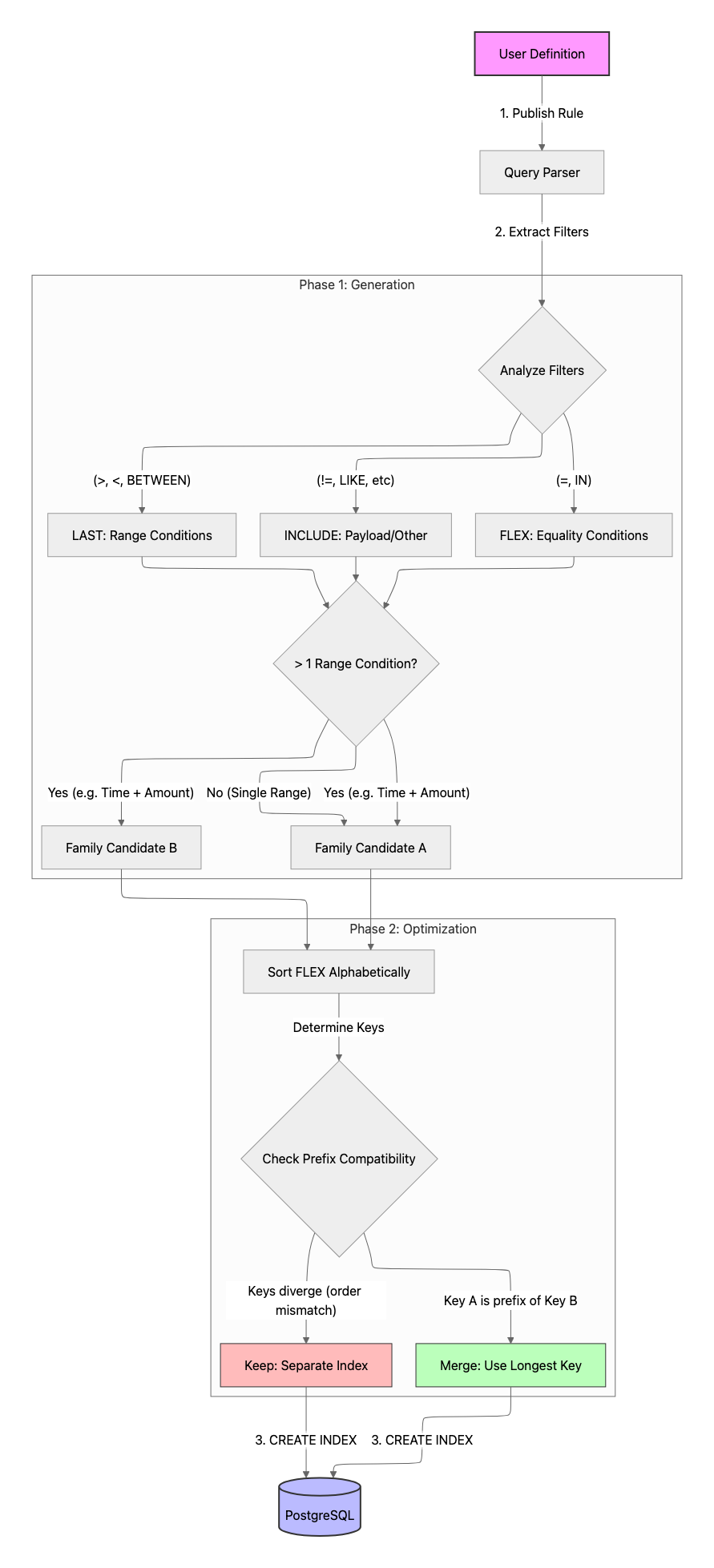
Representing Index Requirements: Fixed, Flex, Last, Include
Many different queries can share the same index. Creating one index per query would be wasteful. To consolidate them, we needed a way to represent what an index needs, without committing to a specific column order too early.
We landed on a structure with four components:
- Fixed: an ordered list of columns that must appear first in the index, in that exact order
- Flex: a set of columns that should appear before the range column, but whose relative order does not matter much, typically equality filters
- Last: at most one column that will carry a range condition (
>,<,>=,<=,BETWEEN); this must appear after all equality columns - Include: columns to put in the PostgreSQL
INCLUDEclause; they are stored in the index for index-only scans but do not affect the B-tree ordering
Mapping this to actual SQL:
- the indexed column list becomes Fixed followed by an ordering of Flex and then Last (if any)
- the
INCLUDElist contains Include columns
Revisiting the earlier example:
SELECT SUM(amount)
FROM org_data.transactions
WHERE account_id = $1
AND transaction_at > $2
AND transaction_at < $3
AND payment_method = $4
AND counterparty_country = ANY($5)we might generate:
- Fixed:
[] - Flex:
{account_id, payment_method, counterparty_country} - Last:
transaction_at - Include:
{amount}
This represents a family of possible indexes, such as:
CREATE INDEX ON org_data.transactions
(account_id, payment_method, counterparty_country, transaction_at)
INCLUDE (amount);
or:
CREATE INDEX ON org_data.transactions
(payment_method, account_id, counterparty_country, transaction_at)
INCLUDE (amount);Any ordering of the Flex set before transaction_at works similarly well for B-tree usage. The choice of a specific ordering, however, is not without consequence. For the system to be idempotent, this choice must be deterministic; we achieve this by sorting the Flex columns alphabetically.
This deterministic but otherwise arbitrary choice is a trade-off. A more advanced strategy could involve micro-optimizations, such as ordering columns by their estimated cardinality (most selective first). Moreover, the chosen order can influence the subsequent merge phase: in complex scenarios, a different permutation might enable better consolidation and lead to a smaller final set of indexes. For our goal of a simple and predictable system, we accept this trade-off.
Phase 1: Building Index Families from Queries
For each aggregate query, we turn its filters into one or more index families (Fixed, Flex, Last, Include).
Step 1: Equality Filters to Flex
Columns constrained by equality (=, IN) are strong candidates for the prefix of the index. We collect them into the Flex set.
For example:
WHERE account_id = $1
AND payment_method IN ($2, $3)gives:
Flex: {account_id, payment_method}
Step 2: Inequality Filters to Last or Include
Range conditions (>, <, >=, <=, BETWEEN) are more delicate. A B-tree index can only effectively support one such column.
Consider:
WHERE account_id = $1
AND transaction_at > $2
AND amount > $3We have:
- equality:
account_id - inequalities:
transaction_at,amount
Ideally, we would pick the more selective inequality to be Last (for example the one that filters out more rows). But we do not introspect data, so we cannot know which is better.
Our decision is: for a query with inequalities on K different columns, we generate K different index families, one for each possible choice of Last:
- Family 1 (favor time):
- Flex:
{account_id} - Last:
transaction_at - Include:
{amount}
- Flex:
- Family 2 (favor amount):
- Flex:
{account_id} - Last:
amount - Include:
{transaction_at}
- Flex:
This may look like it explodes combinatorially, but in practice most aggregates have inequality conditions on exactly one column, rarely two or more.
Step 3: Other Filters to Include
Filters that do not benefit much from B-trees for filtering go to the Include set:
- inequality-like conditions that do not map neatly to ordered scans (for example
!=, someLIKEpatterns) - similarity conditions
- Boolean checks that do not improve selectivity much
We still want to include those columns for index-only scans, so rows can be answered from the index without hitting the base table.
Summary of base construction
For each query:
- put equality filter columns in Flex
- if there are inequalities on K different columns, generate K families:
- each with the same Flex
- one of those columns as Last
- all other filter columns (including other inequalities) in Include
- if there are no inequalities, generate a single family with Flex and Include populated, and Last empty
This postpones the decision of which inequality to favor. We generate all plausible candidates and let the merge phase decide which ones are worth materializing.
Phase 2: merging compatible families
Across all aggregates in a rule version, we end up with a set of index families. Many of them can share a single physical index.
Two families are compatible if there exists a single column ordering and Include set that makes both efficient, given the B-tree rules.
Some intuitive rules:
- if two families share the same Fixed prefix, they are easier to merge
- if one family's Fixed prefix is fully contained in the other's Flex, they may still merge
- if they agree on Last (or one has no Last), merging is more likely to succeed
- if they have different Last columns, they usually cannot merge without sacrificing someone's range efficiency
Example: merging compatible prefixes
The merge logic is based on one index being a valid prefix of another. An index for one family can serve another if the second family's required key columns are a prefix of the first's.
Consider two families with no Last column:
- Family A (from a query on country):
- Flex:
{counterparty_country} - Last:
null - Include:
{}
- Flex:
- Family B (from a query on country and currency):
- Flex:
{counterparty_country, currency} - Last:
null - Include:
{amount}
- Flex:
After sorting the Flex sets alphabetically, the key for A is (counterparty_country) and the key for B is (counterparty_country, currency). Since A's key is a prefix of B's, a single index created for B will also efficiently serve queries for A.
We can merge them into a single requirement by taking the longer key and the union of Include sets:
- Flex:
{counterparty_country, currency} - Last:
null - Include:
{amount}
This generates one physical index:
CREATE INDEX ON org_data.transactions
(counterparty_country, currency)
INCLUDE (amount);This single index works perfectly for queries filtering on just counterparty_country as well as queries filtering on both counterparty_country and currency.
When merging is not possible
Merging is not possible when keys are not prefixes of each other, even if they share columns. This is the critical rule that prevents the creation of inefficient indexes.
Consider these two families:
- Family C:
- Flex:
{account_id} - Last:
transaction_at - Resulting Key:
(account_id, transaction_at)
- Flex:
- Family D:
- Flex:
{account_id, payment_method} - Last:
transaction_at - Resulting Key:
(account_id, payment_method, transaction_at)
- Flex:
These two cannot be merged. The key for Family C is not a prefix of the key for Family D because transaction_at appears in a different position.
An index for Family D would be (account_id, payment_method, transaction_at). A query for Family C filters on account_id and has a range on transaction_at, but provides no filter for payment_method. As per the B-tree primer, this "skips" a column in the index, making it ineffective for the range condition.
Therefore, our heuristic correctly keeps them separate and creates two distinct indexes to ensure both queries are performant. This is one of the places where we accept creating more indexes than theoretically optimal, in exchange for good performance and simple local reasoning.
Trade-offs and alternatives
This approach does not guarantee the absolute minimal set of indexes. The general problem, of finding the smallest set of indexes that makes a set of queries fast, is combinatorial and likely hard in the general case.
We deliberately avoid more sophisticated strategies, such as:
- manual index design by DBAs or engineers based on query plans and statistics
- statistics-driven advisors that look at query logs and propose indexes over time
- materialized views or pre-aggregations with stronger constraints on what aggregates are allowed
Instead, we chose an opinionated, data-agnostic approach that:
- works at rule publish time, with no waiting for statistics
- provides good performance for the common patterns we see (runtime filters over large
transactionstables) - keeps index counts reasonable, though not minimal
In practice, we observe that:
- many aggregates share the same high-cardinality anchor, such as
account_id, plus different additional filters - those aggregates end up consolidated into a small set of shared indexes
- obviously redundant indexes such as
(A, B, C)and(A, B)are mostly avoided when the former suffices
What this buys us
This indexing strategy has been running in production for Marble customers with a wide range of schemas and workloads. It has a few important properties:
- good query performance out of the box: aggregates for new rule versions are backed by appropriate indexes as soon as they go live
- operational simplicity: no manual coordination between rule authors and DBAs, index creation and cleanup are automated and reproducible
- bounded index growth: the merge phase and periodic cleanup prevent unbounded index proliferation, even as rules evolve
Most importantly, it allows fraud and compliance teams to iterate on detection logic in the user interface, while the system handles database details automatically.
Conclusion
Automatic index creation sits at the intersection of user experience and database optimization. By:
- modeling index requirements with a flexible Fixed, Flex, Last, Include structure
- generating index families from queries without data introspection
- merging compatible families into a small shared set
- managing the full lifecycle at rule publish and cleanup time
we have built a system that keeps aggregates fast while staying out of the way of product iteration.
B-tree semantics impose a natural structure on which indexes are useful, especially the "prefix plus one range" rule. Our system exploits that structure. This data-agnostic, heuristic approach gets us remarkably close to the benefits of hand-tuned indexing, without requiring every user to be a database expert.
We believe in building in the open. If you'd like to see how this system is implemented, you can find our work on GitHub.
-Appendix: a concrete example
Let's walk through how five different aggregate queries are consolidated into a final set of three indexes, paying close attention to the B-tree prefix rule.
Input Queries:
1. Query 1: Count of recent transactions for an account.
SELECT COUNT(*) FROM org_data.transactions
WHERE account_id = $1 AND transaction_at > $2;
2. Query 2: Sum of amounts for a specific payment method and account.
SELECT SUM(amount) FROM org_data.transactions
WHERE account_id = $1 AND payment_method = $2 AND transaction_at > $3;
3. Query 3 (with two inequalities): Sum of high-value transactions.
SELECT SUM(amount) FROM org_data.transactions
WHERE account_id = $1 AND transaction_at > $2 AND amount > 5000;
4. Query 4: Count of transactions for a given country.
SELECT COUNT(*) FROM org_data.transactions
WHERE counterparty_country = $1;
5. Query 5 (with IN clause): Total amount from a country across specific currencies.
SELECT SUM(amount) FROM org_data.transactions
WHERE counterparty_country = $1 AND currency IN ('USD', 'EUR');
Step 1: Generating Index Families
This produces six candidate index families:
- Query 1:
Flex: {account_id},Last: transaction_at,Include: {} - Query 2:
Flex: {account_id, payment_method},Last: transaction_at,Include: {amount} - Query 3:
- Family 3a:
Flex: {account_id},Last: transaction_at,Include: {amount} - Family 3b:
Flex: {account_id},Last: amount,Include: {transaction_at}
- Family 3a:
- Query 4:
Flex: {counterparty_country},Last: null,Include: {} - Query 5:
Flex: {counterparty_country, currency},Last: null,Include: {amount}
Step 2: Merging and Finalizing Indexes
The merge process consolidates these six families. The core rule is that one family's index requirement can be satisfied by another's if its key is a prefix of the other's key. We determine the key by alphabetically sorting the Flex columns and appending the Last column.
- Combine Identical Families:
- Families from Query 1 and Query 3a are functionally identical (
Flex: {account_id},Last: transaction_at). We merge them into a single family, taking the union of theirIncludesets. - Result: A single family
Flex: {account_id},Last: transaction_at,Include: {amount}. Key:(account_id, transaction_at).
- Families from Query 1 and Query 3a are functionally identical (
- Group by
Lastcolumn and find merge candidates:- Group 1 (
Last: transaction_at):- Family from Query 1/3a (Key:
(account_id, transaction_at)) - Family from Query 2 (Key:
(account_id, payment_method, transaction_at)) - These are not compatible. Neither key is a prefix of the other. Merging them would create an index like
(account_id, payment_method, transaction_at)which is inefficient for Query 1, as it skips a column. They remain separate.
- Family from Query 1/3a (Key:
- Group 2 (
Last: amount):- Family 3b stands alone (Key:
(account_id, amount)). No other families share itsLastcolumn.
- Family 3b stands alone (Key:
- Group 3 (no
Lastcolumn):- Family from Query 4 (Key:
(counterparty_country)) - Family from Query 5 (Key:
(counterparty_country, currency)) - These are compatible. The key for Query 4 is a prefix of the key for Query 5. We can satisfy both with a single index.
- Result: A merged family
Flex: {counterparty_country, currency},Last: null,Include: {amount}.
- Family from Query 4 (Key:
- Group 1 (
This process results in four final indexes:
Index 1 (from Query 1 & 3a):
CREATE INDEX ON org_data.transactions
(account_id, transaction_at)
INCLUDE (amount);
Index 2 (from Query 2):
CREATE INDEX ON org_data.transactions
(account_id, payment_method, transaction_at)
INCLUDE (amount);
Index 3 (from Query 3b):
CREATE INDEX ON org_data.transactions
(account_id, amount)
INCLUDE (transaction_at);
Index 4 (from Query 4 & 5):
CREATE INDEX ON org_data.transactions
(counterparty_country, currency)
INCLUDE (amount);
From five queries, the system correctly derived four indexes that cover all needs efficiently by strictly adhering to the B-tree prefix rule. Of the four, one (index 3) could be removed by changing the heuristics in a simple way.

Pascal Delange

